This page has been developed by B. Haesler, RVC
1. The economic evaluation of surveillance in relation to intervention and disease mitigation
In the three variable relationship of disease mitigation, surveillance and intervention, the latter two can either be economic complements or substitutes. Surveillance and intervention resources as complements means that they always go together in a given ratio and can be considered to be one input, for example as seen in a testing (surveillance) and culling (intervention) strategy. Surveillance and intervention as substitutes means that using more of one input will allow the use of less resources for the other to achieve the same loss avoidance. The most prominent example here is early warning surveillance that aims to enable early response and containment of disease.
For optimal efficiency, the combined cost of surveillance and intervention should be minimised for a given disease mitigation objective. A disease mitigation objective is typically expressed as a reduction in prevalence or incidence (e.g. “reduce prevalence of disease x in population y by 10%”, “eradicate disease from population z”); both are technical measures of disease occurrence. If the value of loss avoidance is of interest (e.g. in a cost-benefit analysis), such prevalence or incidence reduction must be translated into the corresponding economic values of loss avoidance (Häsler and Howe 2012).
Any given level of value losses avoided may be obtained from different combinations of surveillance and intervention effort. In general, allocating more resources to surveillance should lead to better information about a disease threat which allows more targeted intervention. For example, identification of holdings or areas infected or at risk of disease, allows focusing treatment on those populations instead of choosing a blanket approach. Similarly, detecting a disease early through surveillance enables intervening at a point when the losses due to animal disease and disease spread are still limited, and resources required to tackle cases are lower than later in an outbreak.
For any disease of interest, it is therefore necessary to consider the technical trade-offs between surveillance and intervention that lead to distinct levels of loss avoidance, as described in detail elsewhere (Howe, Häsler, and Stärk 2013). Figure 1 summarises the key principle: curves A1 and A2 represent two hypothetical levels of loss avoidance, which can be achieved by multiple combinations of surveillance and intervention. They illustrate the possibility of substitution between surveillance and intervention for two out of potentially very many feasible levels of avoided losses. The loss avoidance in curve A2 can be achieved by either doing a lot of surveillance and limited intervention (S* and I*) or limited surveillance and a lot of intervention (S° and I°).
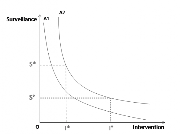
Figure 1: The curves A1 and A2 describe two defined levels of loss avoidance (where A1<A2) that can be achieved by varying levels of surveillance (S) and intervention (I). From Häsler et al. 2013: Surveillance and Intervention Expenditure: Substitution or Complementarity between Different Types of Policy.
When including budget lines Figure 2 (i.e. lines that represent all combinations of surveillance and intervention that, when added up, have the same total amount of mitigation expenditures), the least-cost combinations of surveillance and intervention for the highest possible level of loss avoidance can be identified. The least-cost combination of surveillance and intervention use for this budget line is where the line touches curve A2 (marked with a dot). Other combinations along the budget line are possible as well, but must yield lower values of loss avoidance (marked with stars in Figure 2).
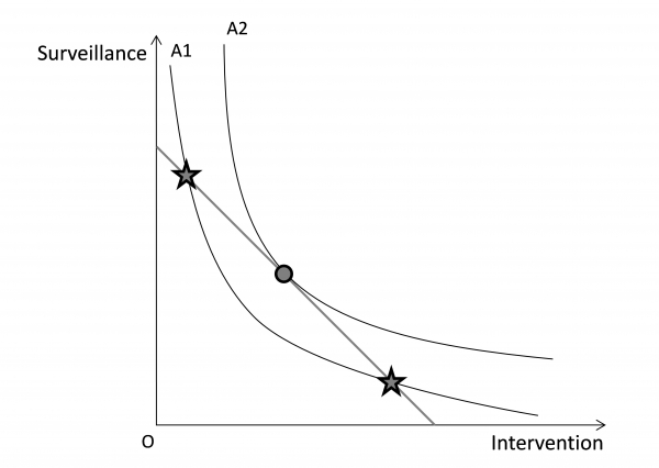 Figure 2: A higher level of loss avoidance (curve A2) can be achieved with the ideal combination of resource use (where the budget line touches the loss avoidance curve, marked with a dot).
Once least-cost combinations are plotted in relation to levels of loss avoidance (A1 to An), an expansion path can be identified, i.e. a line through all the tangent points on loss avoidance curves with the corresponding budget lines for surveillance and intervention. The economic optimum or in other words the maximum net benefit for society can be found where the marginal loss avoidance (i.e. marginal benefit) equals the marginal costs on the expansion path. To identify this economic optimum for disease mitigation, it is necessary to understand the technical relationships between loss avoidance, and the use of surveillance and intervention resources and the valuation (pricing) of the resources. The valuation is used to translate loss avoidance and resource use into monetary values such as benefits and costs. Then, least-cost combinations for surveillance and intervention can be determined and the least-cost combination(s) identified that are consistent with the avoidance loss that maximises economic welfare.
2. Common economic evaluation methods applied to surveillance
2.1 Cost-effectiveness analysis (CEA)
Given resource and technical constraints, there is a demand in the surveillance community to include intermediate outcomes (e.g. sensitivity of a system) instead of final outcomes (e.g. number of sick animals avoided) in CEA. The attractiveness of such an approach is that it apparently avoids the need for valuation of the outcomes and therefore can save resources in the analysis. For instance, an effectiveness measure such as timeliness may be considered to be a proxy for the final outcome or benefit, such as loss avoidance and reduced intervention expenditures due to earlier outbreak detection (which would be measured explicitly in a cost-benefit analysis). However, CEA of surveillance can inform resource allocation meaningfully only if the effectiveness measure has an interpretable value. For example, the value of timeliness may have been established in studies of past outbreaks to know that each day of earlier detection of a highly pathogenic avian influenza (HPAI) outbreak resulted in the avoidance of losses worth £100,000. In such a case, a cost-effectiveness ratio of a surveillance system to early detect HPAI expressed as costs/days of earlier detection can be easily interpreted. However, without this information, effectiveness measures like time of introduction of disease until detection or the probability of detecting an outbreak are not informative in a CEA.
Therefore, before conducting a CEA, it is necessary to think carefully about how the findings can be interpreted and whether the value of an effectiveness measure can be compared to the additional costs.
Effectiveness measures used in CEA of surveillance to date include global evaluation score of the surveillance system, probability of introduction or transmission of the disease, number of infected farms at the end of the epidemic, number of herds detected by the surveillance, and sensitivity of detection. A wide range of other epidemiological performance indicators for surveillance are available, such as timeliness, negative predictive value, positive predictive value, bias, precision, or false alarm rate (Hoinville et al., 2013). There are two main challenges associated with the use of such effectiveness measures in a CEA of surveillance:
1) The use of a wide range of surveillance effectiveness measures limits standardisation and comparability across programmes; and
2) Certain effectiveness measures cannot be valuated intuitively; it is therefore difficult for decision-makers to choose a cost-effectiveness threshold such as those used for human health
The issue is further complicated by the overlap between performance indicators. Moreover, some common performance indicators are only applicable to specific surveillance objectives and/or contexts. For instance, negative predictive value is suitable for surveillance that aims to demonstrate freedom from disease, whereas sensitivity is relevant for surveillance that aims to early detect disease or to find cases.
In any situation, the choice of a cost-effectiveness threshold by decision-makers depends on the perspective of the analysis (e.g. societal or sectoral), the value people attribute to the effectiveness outcome, their risk attitude and resource availability (Owens, 1998). These factors will result in setting different cost-effectiveness thresholds for the given outcome.
Moreover, the type of effect measure to include in a CEA depends on the context and surveillance objective, which in turn is driven by the mitigation objective (Häsler, Howe, and Stärk 2011). For example, the context may be defined by legal, social, or political factors, the disease situation in the country and the availability of technical expertise and capacity. In a low or middle income country with endemic disease, the ability of a surveillance system to identify infected animals in order to target them for intervention will be key, while in a high income country that has controlled major diseases the timeliness of surveillance in terms of early detection may be of higher priority.
Epidemiological information is often needed to determine surveillance effects. Commonly, a surveillance system will be expected to fulfil an objective that results in a numeric outcome. For example, the objective may be to find cases in a population for disease mitigation and the associated effectiveness measure may be defined as “number of infected animals identified” (which may, for example, be a proxy measure of successful mitigation and therefore animal mortality avoided).
There are three types of CER corresponding to different uses:
Average cost-effectiveness ratio (ACER)If we are looking at surveillance options that are non-competing (i.e. you can implement them in parallel) or we are only looking at one single surveillance option, the following approach applies: Calculation of the average cost-effectiveness ratio (=divide the net cost of surveillanceby the effectiveness) of each option and then gradual implementation of options starting from the one with the lowest cost per unit outcome until the budget is used (Table 1).

NOTE: We need to use SAME effectiveness metric for the outcomes for all options.
Table 1: Example ACER
| Surveillance | Number of brucellosis cases detected | Net Cost | ACER |
| A) Slaughterhouse surveillance | 50 | £1000 | £20/brucellosis case detected |
| B) Fallen stock surveillance | 3 | £300 | £100/brucellosis case detected |
| C) Bulk milk surveillance | 40 | £1200 | £30/brucellosis case detected |
Hence, implement first A, then C, then (if you have enough money) B.
It is difficult to think of examples where we would start implementing several surveillancesystemsin parallel that have the same effectiveness metric. However, it is different for components, where an approach could be to add further components until the budget is used up.
Incremental cost-effectiveness ratio (ICER)
More often we are faced with a situation where we have several surveillance options that are competing for the same resources and we can choose only one - in other words they are mutually exclusive (e.g. use risk-based surveillance or conventional surveillance). This could be of interest when looking at replacing the present surveillance system with a new system or when assessing a set of options when planning a new surveillance system.

For this, the incremental cost-effectiveness-ratio (ICER) should be used, which allows determining the marginal or incremental cost for an additional unit of outcome measure when choosing between different surveillance options. It measures the additional cost per additional outcome (Table 2).
NOTE: We need to use SAME effectiveness metric for all options.
Table 2: Example ICER
| Surveillance | Number of abortions avoided | Net Cost |
| S (status quo) | 18 | £300 |
| W | 20 | £500 |
| X | 21 | £400 |
| Y | 30 | £2000 |
| Z | 25 | £1000 |
In order to make the appropriate comparisons, we first need to order the interventions from least expensive to most expensive or in the order of effectiveness. This gives us the following table:
Table 3: Example ICER continued – rank in terms of cost
| Surveillance | Number of abortions avoided | Net Cost |
| S (status quo) | 18 | £300 |
| X | 21 | £400 |
| W | 20 | £500 |
| Z | 25 | £1000 |
| Y | 30 | £2000 |
We can rule out W, because it is strongly dominated by surveillance X, which costs less and yields a better outcome.
The incremental cost is found by calculating the additional cost of the more expensive surveillance relative to the surveillance that is less expensive. In our example, incremental cost between X and S = (Cost Z – Cost S) = £400-£300 = £100. Similarly the additional health benefit (our effectiveness) is simply the additional health benefit of implementing a surveillance option relative to the option that is less expensive. In our example, incremental benefit = (No. abortions avoided X – No. abortions avoided S) = 3 additional abortions avoided. Finally, divide the incremental cost by the incremental benefit (=£33/additional abortion avoided). This means that if we chose to implement X in place of S, it would cost £33 per additional abortion avoided than we would get from implementing X.
The incremental cost-effectiveness ratio of each intervention is then found by comparing it to the slightly more expensive (or next most effective intervention if ordered by effectiveness) option, hence we need to compare option Z with option X and Y with option Z next. For X and Y this is (£1000-£400)/(25-21)=£150/additional abortion avoided and for Y and Z (£2000-£1000)/(30-25)= £200/additional abortion avoided.
Table 4: Example ICER continued – the ICER calculated
| Surveillance | Number of abortions avoided | Net Cost | ICER (£/additional abortion avoided) |
| S (status quo) | 18 | £300 | - |
| X | 21 | £400 | 33 |
| Z | 25 | £1000 | 100 |
| Y | 30 | £2000 | 200 |
The final table indicates the surveillance options and their incremental cost-effectiveness ratios. It is now up to the decision maker to choose among the surveillance options by deciding how much an abortion is worth. If an abortion is not worth even £33 to the decision-maker, then none of the options generate sufficient value to be adopted. If an abortion is worth more than £200, then surveillance Y should be adopted. For example, an abortion in cattle in the UK costs a farmer roughly around £1000; hence option Y would be recommended. This demonstrates that an effectiveness measure needs to be interpretable. Therefore it is important to carefully reflect every time on what the effectiveness measure tells us and how it can be interpreted.
Marginal cost-effectiveness ratio (MCER)The marginal cost-effectiveness ratio assesses the specific changes in cost and effect when a programme isexpanded or contracted(e.g. the additional costs of surveying 10 more farms without changing the surveillance design). This helps to identify the point of optimal level of a surveillance system where the largest overall benefit is produced – it therefore follows the same basic concept as optimisation. It defines the level where most health effects are reached at lowest costs according to the following equation:

A special form of CEA in surveillance, which effectively falls between traditional CEA and least-cost analysis, is the situation where the surveillance effect needs to achieve a minimum threshold and all options above this threshold are treated to be equal in terms of their effectiveness (in fact a binary output – threshold reached yes/no). Examples are surveillance demonstrate with a confidence of 95% that a country is free from a disease or achieve a sensitivity of detection of 80%. For this economic evaluation, it is necessary to first establish the equal effectiveness using relevant methods. Next, the costs of all equal options can be calculated and the options be ranked according to costs. By adopting the least-cost of equal surveillance options, the highest net benefit can be achieved. An example where this approach can be of interest is where outcome-based standards require a minimum effectiveness and several surveillance designs may be possible. In such a case, it is necessary to assess whether the different designs achieve the required outcome and to calculate the surveillance costs for all those that do achieve the target. The surveillance option with the least cost is the one that achieves the highest economic efficiency and is the one that should be chosen if only economic considerations apply.
2.2 Least-cost analysis
Least-cost analysis aims to identify the cheapest among different possible options producing the same outcome. In this type of analysis, the cost is the dominant determining factor in a choice between different options, the outcome or value of the outcome is fixed. The valid application of the method depends on establishing that the cost is indeed the determining factor and that the effect is the same for the surveillance options to be compared.
In its strictest sense, least-cost analysis of surveillance applies where the surveillance design and protocol is given by for example legislation (e.g. definition of the types and number of farms and samples is provided, laboratory testing and analysis procedures are described), it can be expected that the surveillance component achieves the desired effect. Different surveillance options to be compared then can only look at changes in the implementation of the surveillance (e.g. use cheaper test tubes from a different manufacturer, use synergies between programmes) and select the option that complies with the given requirements at minimum cost.
Another type of least-cost analysis, which effectively falls between traditional CEA and least-cost analysis, is the comparison of different surveillance options that achieve a defined target in terms of effectiveness (e.g. demonstrate with a confidence of 95% that a country is free from a disease or achieve a sensitivity of detection of 80%). For this economic evaluation, it is necessary to first establish the equal effectiveness using relevant methods. Next, the costs of all equal options can be calculated and the options be ranked according to costs. By adopting the least-cost of equal surveillance options, the highest net benefit can be achieved. An example where this approach can be of interest is where outcome-based standards require a minimum effectiveness and several surveillance designs may be possible. In such a case, it is necessary to assess whether the different designs achieve the required outcome and to calculate the surveillance costs for all those that do achieve the target. The surveillance option with the least cost is the one that achieves the highest economic efficiency and is the one that should be chosen if only economic considerations apply. Consequently, this type of least-cost analysis requires assessment of the effect as a first step and consideration of the costs of options that achieve a defined threshold, which means that is can also considered to be a special type of CEA.
2.3 Cost-benefit analysis
Cost-benefit analysis (CBA) aims to evaluate, in monetary terms, all types of costs and benefits of surveillance, direct and indirect, market and non-market values, in order to find out if it generates a positive net value. In CBA, direct costs and benefits are related to the direct effects resulting from animal health surveillance (e.g. resource use, animal health), while indirect costs and benefits are related to its wider positive or negative external effects (externalities), e.g. on the whole economy, on human health or on the general social welfare, on the environment. Some costs and benefits originate from goods and services created by surveillance and are valued through the market, i.e. their value is expressed through a market price. But some inputs, goods and services are not exchanged in a market (e.g. absence of pain or suffering) and therefore have no market prices and their monetary values have to be deducted indirectly through methods such as contingent valuation. A major advantage of CBA is that it is applicable to a wide range of problems and that it provides decision-makers with an objective tool, as the costs and benefits are expressed in monetary terms. Drawbacks of conventional SCBA are that price effects and linkages across sectors are often omitted and that it is not ideal for capturing longer-term dynamic effects (Rich et al., 2005).
Capturing and quantifying all the costs and benefits of surveillance is critical in CBA. Key steps are to identify surveillance options to be compared (note that an option can be not to do anything), to identify the steps requiring resource used, to identify all the potential losses incurred by the disease for all options, to measure and value the costs and the benefits (losses avoided) in the same monetary unit, and to compare the costs and benefits between the different surveillance options. Three measures are commonly used in CBA, which are economic acceptability criteria used to determine whether the benefits stemming from a mitigation policy at least cover its costs, thus making a strategy justifiable: net present value (NPV), benefit-cost ratio (BCR) and internal rate of return (IRR); they all have their strengths and weaknesses.
When conducting a cost-benefit analysis of surveillance, it is important to consider the following:
- Loss avoidance (=benefits) is only possible if surveillance and intervention are considered together. Surveillance is inextricably linked to intervention as explained above and so the assessment of the benefit is meaningful only when interpreted as part of the overall disease mitigation process. This is corroborated by the fact that existing economic assessments of surveillance generally relate surveillance activities to the probability of a disease outbreak and its consequences including response costs (e.g. Carrasco et al. 2010; Kompas; Moran and Fofana 2007). Therefore, the cost-benefit analysis must include data on intervention and surveillance and the mitigation outcome.
- The counterfactual (or baseline, i.e. the situation without the mitigation programme in question) can be highly dynamic depending on the disease in question. Often, at least one option is a hypothetical option, which means that predictions need to be made on the effects by for example using epidemiological simulation models. This relates close to the quantification of benefits.
- The timeline of the programme to be evaluated needs to be chosen carefully taking into account the planning, implementation and evaluation horizon. For example, if the endpoint of the programme is the elimination of disease from a population, the analysis will not have to take into account post-elimination surveillance costs to monitor freedom from disease. However, if the time span of the investment to be assessed includes the post-elimination period, the costs of long-term surveillance to sustain the free status and the costs of potential re-incursions of disease will also have to be considered (Häsler, Howe, and Stärk 2011).
2.3.1 Economic acceptability criteria
The net present value (NPV), benefit-cost ratio (BCR) and internal rate of return (IRR) are three economic acceptability criteria used in CBA and are calculated as follows:
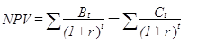
TheNPVis the difference between the sum of the present value of the benefits (B) and the sum of the present value of the costs (C) and should be positive for an investment to be worthwhile (t=time in years; r=discount rate):
TheBCRis the ratio between the sum of the present value of benefits and the sum of the present value of costs and should be ≥1 for an investment to be worthwhile:

TheIRRis the discount rate that will make that net present value zero. If the IRR is bigger than the minimal acceptable discount rate, the investment is considered worthwhile. It is calculated by solving for r such that:

In summary, CBA compares the total discounted benefits of a project in monetary units with its total discounted costs in monetary units and recommends the implementation of the project if the benefits exceed the costs. It includes the definition of the useful life of the project or programme, estimating physical units of benefits (e.g. losses avoided) and costs (e.g. mitigation resources used), translation of the physical units into economic values, the conversion of future values into present values by discounting, and finally the calculation of the choice criteria described.
2.3.2 Strengths and weaknesses of economic acceptability criteria
All three choice criteria provide different information and it is therefore recommended to look at the three of them in conjunction (Gittinger 1982):
Weaknesses:
- Big projects give high NPVs, there may be several other smaller projects that yield higher BCRs and IRRs. Much depends on whether the one large projects replaces a smaller higher yielding project (they are exclusive) or whether the smaller project can be applied several times or alongside other smaller and higher yielding projects. In the animal health field, a large project might be a nationwide stamping out. Smaller projects might be herd by herd decisions on vaccination and/or stamping out. The projects would be exclusive if a government decision had been taken to go for stamping out. They would be compatible if farmers could choose.
- BCRs change if some costs are netted out (subtracted) from benefits before overall benefits and costs are added up and the BCR calculated. This usually increases the value of the BCR. It happens often in the vet field, because there is a tendency to look at the costs of the government vet services or of a project as against the increase in income to farmers/livestock producers. But livestock producers have their own costs (time, extra costs of keeping livestock, cost of applying new disease control measures) and these should, strictly speaking, be added to government/project costs. However, they are often subtracted from the extra livestock output to give net benefits or income to producers and these are treated as ‘the benefits’.
- IRRs can be artificially high - over 100% - for projects where there is very little ‘up-front’ expenditure. This happens often in the vet field where a regular intervention yields a regular benefit without a lot of investment at the start – e.g. a vaccination programme. (This is the opposite of the disease eradication scenario, where a lot of expenditure up front yields benefits in perpetuity, but a relatively low IRR). Of course IRRs can’t be calculated at all if B > C every year of the project.
Strengths
- NPV tells you how much money you gain, over and above your minimum cut off (the discount rate)
- BCR is unaffected by project size
- IRR gives you your average annual % return over the life of the project, a neat measure. It means you can be less definite about what your cut-off or minimum acceptable % return is = the discount rate. Both NPV and BCR depend on the discount rate.
2.3.3 Quantifying surveillance benefits
The important concept of loss avoidance is illustrated here with an example of early warning surveillance, where detecting disease early is expected to lead to a more rapid response (e.g. implementation of outbreak control measures) relative to the time of occurrence of the index case. Earlier in the outbreak, the losses already generated by the disease are smaller than at a later time. As a consequence, less spread means that the costs of intervention measures required are smaller than later in the outbreak with more animals and/or holdings being affected (Figure 3).
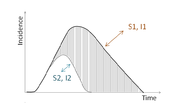 Figure 3: Comparison of two surveillance options (S1 and S2) and their associated interventions (I1 and I2) in a situation where S2 leads to earlier detection of disease and I2 to effective disease control. The hatched area represents the losses avoided with the more effective combination of S2 and I2.
To estimate the value of losses avoided, it is necessary to identify the effects in the animals or holdings affected as well as the effect of potential externalities. The losses can then be estimated by multiplying the number of animals of a certain type or species (e.g. dairy cows) suffering from a disease impact (e.g. reduction in milk yield) by the lost physical production coefficient (e.g. rate of reduced milk yield in dairy cows) and the price coefficient related to the disease impact (e.g. production price per litre cow milk). All disease effects need to be “translated” from a technical perspective into a value perspective in this way and summed up. The resulting difference in losses between two strategies is the benefit.
For surveillance that aims to detect cases of a specified condition in order to implement an intervention, the same logic applies. Figure 4 illustrates two levels of surveillance with their associated interventions for three different baselines of decreasing, stable and increasing prevalence. In each case, the surveillance and intervention costs need to be estimated and compared to the estimated associated loss avoidance to determine the economic efficiency of the mitigation strategy. The strategy to be preferable from an economic point of view is the strategy that creates the largest net benefit, i.e. where the (positive) difference between loss avoidance and combined surveillance and intervention costs is largest.
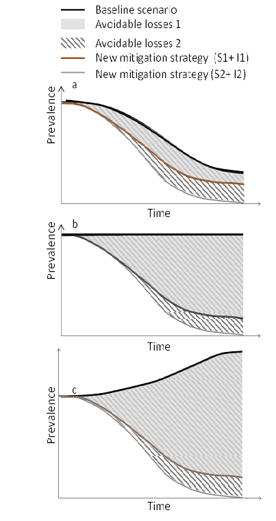 Figure 4: Comparison of two surveillance options and their associated interventions (S1&I1 and S2&I2) in a situation where the mitigation option 1 leads to disease reduction and the mitigation option 2 to disease elimination. A-c represent different baseline scenarios with decreasing, stable and increasing prevalence. The grey and hatched areas represent the losses avoided when the new strategies are compared to the baseline.
Because the impact of surveillance cannot be measured directly as a mitigation outcome, it is only possible to quantify the loss avoidance resulting from the combination of surveillance and intervention and to compare it to the expenditures for surveillance and intervention. Therefore, it is recommended to calculate a residual margin over intervention cost which constitutes the maximum additional expenditures potentially available for surveillance without the net benefit from mitigation overall becoming zero. This margin can then be compared to the expenditures of various surveillance options and the one maximising the net benefit would be the best from an economic point of view. An illustration of this concept can be found in Häsler et al. (2012).
Using intermediate outcome proxy measures for the benefit (e.g. number of cases detected) for inclusion in a cost-effectiveness analysis is only justifiable when a clear correlation between the intermediate outcome and the benefit is firmly established through empirical research. Otherwise, the case detection capacity of a surveillance system is non-interpretable from an economic point of view. A logic model can help to establish the relationships between intermediate and final outcomes. For example (Figure 5):
 Figure 5: A schematic logic model to illustrate the steps that leads from surveillance to a reduction of foodborne illness in humans.
In the example depicted in Figure 5, if the aim of mitigation is to avoid human cases (the value of such avoidance can be quantified) and only the case detection capacity of surveillance is to be assessed and compared to the costs of the surveillance, the link between the intermediate outcome (disease detection) and the final outcome (reduction in human cases) needs to be established.